p-value p-rimer

The much-maligned p-value is a concept first encountered when learning about probability distributions, and later when learning about statistical hypothesis testing. These are my notes from a week-long deep dive into p-values and hypothesis testing.

Definition

Assuming the null hypothesis (along with all other model assumptions) is true, the p-value is the probability of getting a result at least as extreme as the one observed.

More generally, it is

... the probability under a specified statistical model that a statistical summary of the data (e.g., the sample mean difference between two compared groups) would be equal to or more extreme than its observed value. -- American Statistical Association 2016 statement

This "statistical summary" is usually a test statistic (e.g. t-statistic) that measures departures from the null hypothesis.

p can be used as a measure of how compatible the observed data are with the model used to compute it. 0 = totally incompatible, 1 = totally compatible.

If the model and the null hypothesis are correct, then p will vary randomly in a uniform distribution (but only for continuous data as shown in Murdoch et al 2008) and take on values less than $\alpha$ about 100*$\alpha \%$ of the time (Greenland 2019). This is because if the null and the model assumptions are correct, the p-value reflects random error from study to study.

History of the p-value

Summary of Kennedy-Shaffer 2019.

The p-value is widely attributed to Karl Pearson, who introduced it with his Chi-squared test in 1900. However, similar formulations of the same concept can be found as early as 1710 in John Arbuthnot's examination of the male:female birth ratio. In the 1800s, mathematicians such as Laplace, Poisson, and Cournot used similar techniques in their work.

1902: William Palin Elderton publishes tables of p-values for Pearson's Chi-squared distribution.

1908: William Gosset ("Student") publishes his t distribution with similar tables of probabilities.

1922: Ronald Fisher expands on the use of p-values in three monographs:

i) On the Mathematical Foundations of Statistics

Likelihood and maximum likelihood estimation

ii) On the Interpretation of χ2 from Contingency Tables, and the Calculation of P

Calculating p-values from contingency tables using the $\chi^2$ distribution

iii) The Goodness of Fit of Regression Formulae, and the Distribution of Regression Coefficients

Significance testing on regression coefficients using the t distribution

Statistical Methods for Research Workers

Fisher fleshed out the details of p-values in his 1925 book, Statistical Methods for Research Workers, and introduced the (in)famous 0.05 threshold for significance. These tables allowed scientists to look up values easily without tedious manual calculations. The tables inverted the order of Pearson's and Gosset's tables—they let you look up the test statistic based on a range of pre-specified p-values, instead of the other way round. This also had the effect of emphasising the concept of levels of significance.

Brief notes on hypothesis testing

p-values are the focal point of modern null hypothesis significant testing (NHST). NHST is borrows key elements from Ronald Fisher's original significance-testing framework and Jerzy Neyman and Egon Pearson's hypothesis-testing approach. Not included: details of the famous squabbles that erupted among these esteemed granddaddies of statistics.

Fisher (significance testing)

• If the data are rare under the model (small p), then this is evidence against the null hypothesis.
• The value of p is a continuous measure of evidence against the null. The smaller the value, the stronger the evidence against the null.
• Influences the scientist's belief about the truth as part of an inductive process (particular → general).
• Terms can be determined post hoc.

Steps

1. Choose a statistical test e.g. chi-squared test, t-test.
2. Define the null hypothesis—not necessarily a hypothesis of zero effect. "Null" refers to the objective of nullifying a specific hypothesis.
3. Calculate the theoretical probability, p, of the observed results given the null hypothesis.
4. Assess statistical significance - there is no "bright line" threshold. If p is small, either a rare event has happened, or the null hypothesis is false.

Neyman-Pearson (hypothesis testing)

Without hoping to know whether each separate hypothesis is true or false, we may search for rules to govern our behaviour with regard to them, in following which we insure that, in the long run of experience, we shall not be too often wrong. -- Neyman and Pearson (1933)

• Testing is a way to choose between the null hypothesis and an alternative hypothesis.
• Allows us to minimise long-term error rates—meant for long-run sequences of repeated experiments (whereas Fisher's p is from a single experiment).
• Makes a distinction between inductive belief and behaviour: the scientist using the Neyman-Pearson framework can decide to take actions based on accepting a hypothesis without necessarily believing it is true. Whereas Fisher favoured an inductive approach (particular → general), Neyman and Pearson adopted a deductive stance (general → particular).
• Aids pragmatic decision-making.
• Good for processes that involve repeated sampling (e.g. quality control).
• Terms need to be determined a priori.

Steps

1. Define an alternative hypothesis with an effect size of interest.
2. Choose a statistical test with suitable power. Power = probability of rejecting a false null hypothesis (= sensitivity) i.e. the probability of not making a false negative error.
3. Evaluate these two types of errors:
   • Type I: Rejecting $H_0$ when $H_0$ is true (false positive), denoted by $\alpha$
   • Type II: Accepting $H_0$ when $H_0$ is false (false negative), denoted by $\beta$ ($= 1 - power$)
4. Optimise the decision rule by minimising type II error rate where the maximum tolerable (e.g. based on cost) type I error rate is set to a significance level $\alpha$ (determined a priori)

$\alpha$ is an arbitrary value set a priori, $\beta$ is controlled by choosing a sample size based on power calculations. See Scucz and Ioannidis 2017.

See Lehmann 1993 for a useful comparison of the Fisherian and Neyman-Pearson frameworks.

Nitpicky note: Lehmann equates the Type I error rate to the significance level but Hubbard (2004) and Greenland (2019) say this is wrong—significance is a Fisherian construct and is determined by p.

Alpha

$\alpha$ is not the actual type I error rate. $\alpha$ is set a priori as a maximum tolerable type I error rate; the actual error rate will deviate if the data are not continuous or if the assumptions of the model and test are not perfectly valid. See Greenland 2019.

If the null is true, over many experiments, you would (falsely) reject it $\alpha$ proportion of times. It is an upper bound of the type I error rate.

Note also that $\alpha$ (false positive rate) is not the false discovery rate.

False positive rate = No. of false positives (rejecting $H_0$) / No. of negative results ($H_0$ is true)

False discovery rate = No. of false positives / No. of all positive results

See also this Cross Validated thread.

Null hypothesis significance testing (NHST)

An anonymous hybrid consisting of the union of the ideas developed by Ronald Fisher, on the one hand, and Jerzy Neyman and Egon Pearson, on the other. -- Hubbard 2004

• Comparing p to $\alpha$ was not what Fisher or Neyman and Pearson had intended (whether this fact is important is debatable IMO).
• p is a feature of the data, $\alpha$ is a feature of the experimental procedure.
• "Never accept the null hypothesis" comes from Fisher. In Neyman-Pearson's framework you accept either the null or the alternative.
• Dichotomous results: "significant" or "not significant"

Steps

1. Compute p, report its exact value and its nominal level of significance (highly significant, marginally significant etc.) ← Fisher
2. Compare p to a threshold level ← N-P
3. If p $\leq$ threshold then reject the null and claim evidence of an effect

Cross Validated: Is the "hybrid" between Fisher and Neyman-Pearson approaches to statistical testing really an "incoherent mishmash"?

Why 0.05?

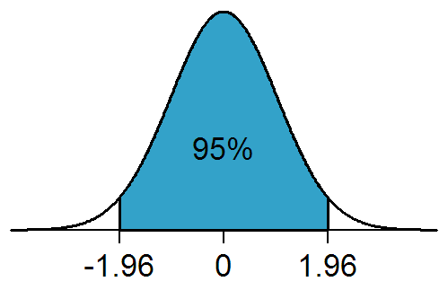
In a standard normal distribution, a two-tailed p = 0.05 corresponds to about two standard deviations (1.96) from the mean. 5% would have been an arbitrary but socially acceptable criterion for how strong evidence should be before we take it seriously (Stigler 2008)

Factors affecting significance

See Greenland 2019 for details.

Effect size

Larger effect size → larger deviation → larger test statistic → smaller p-value

Precision

The more precise the estimate, the greater the evidence against the model produced by a deviation from a model prediction

Measurement precision

Higher precision → smaller standard error → larger test statistic → smaller p-value

Sample size

Larger sample → higher precision → smaller standard error → larger test statistic → smaller p-value

The problem with large samples

In very large samples, the p-value becomes overly sensitive to small deviations from the null or the model assumptions.

Common misconceptions

Greenland et al 2016 contains a concise and illuminating summary of common pitfalls in NHST.

p = Probability that the null hypothesis is true

p is calculated by assuming that the null hypothesis is true.

p = Probability that the observed results occurred by chance

p is calculated assuming that chance alone produced the effect (null hypothesis is true).

This quantity is instead given by the false discovery rate (= false positive / all positives)

Statistically significant = practically significant

Practical significance depends on the effect size and other contextual factors such as implementation costs, number needed to treat, adverse effects etc. A significant p-value tells you there is likely to be an effect, without giving direct information about the magnitude of the effect.

p = significance level

The significance level is $\alpha$, which is determined a priori. p is an a posteriori value calculated from the data.

"p > 0.05" = no effect observed/no association/no evidence for effect

As long as p < 1 there is some incompatibility with the model that assumes no effect.

p is the probability of a type I error

Cross Validated: What is the Relationship between p-values and Type I Errors?

If $p > \alpha$, then the probability of a type I error is zero because we wouldn't reject the null hypothesis in the first place.

If $p < \alpha$ (we reject the null hypothesis) and the null hypothesis is true, then the probability of a type I error is 1.

The type I error rate is a long-run probability over repeated experiments. A single p-value from a single experiment is not the same things as this long-run error rate.

Advantages of using p-values

• Simple Quick heuristic to help distinguish true effects from random noise—this entire post highlights how the p-value is the opposite of simple.

Arguments against p-values

• The p-value has been blamed in part for the reproducibility crisis in biomedical research due to p-hacking.
• Promotes false equivalence between a lack of statistical significance and "no difference", "no association".
• Draws attention away from the effect size.
• Dichotomous use of p (> 0.05 -> not significant, <= 0.05 -> significant) is silly, especially because "statistically significant" and "not statistically significant" is often not statistically significant (Gelman and Stern 2006).

Calls for reform

• Nuzzo 2014 Nature editorial on p-values.
• Amrhein et al (2016) in Nature against statistical significance.
• 2019 editorial in The American Statistician advocating against "statistical significance".

... and many more.

How should p be used?

• Not as a dichotomous, reductive decision aid.
• In combination with effect sizes (Gosset had raised this in response to Fisher's framework).
• In combination with confidence intervals, which include other effect sizes that may be important. Consider the implications of these effect sizes.
• Include the p-value prediction interval (similar to a confidence interval for effect size).
• In the context of study design, measurement quality, validity of assumptions, external evidence.
• Report exact values. p = 0.04 is not the same as p = 0.01 and should not be lumped together by merely stating p < 0.05
• As a screening test for multiple hypotheses in high-throughput studies, such as GWAS and gene expression studies Huber 2016

p-oetry

This list of bullshit phrases selling p-values is absolutely mesmerising.

Useful discussions on Cross Validated

• What is the meaning of p values and t values in statistical tests?
• Are smaller p-values more convincing?
• How much do we know about p-hacking "in the wild"?
• ASA discusses limitations of p-values - what are the alternatives?
• Why do people use p-values instead of computing probability of the model given data?

Day 34 of #100DaysToOffload

← Home